autoplot para series de tiempo

estacional <- read.csv("Estacionalidad.csv", sep = ",", dec = ".", header = T)

La función autoplot() de la librería ggbio trabaja bajo ggplot2 y nos permite realizar mejores gráficos para la modelación de series de tiempo.

Primero debemos convertir el objeto de la serie de tiempo a un objeto ts para que se pueda cargar en autoplot(). Esto es muy común en la modelación de las series de tiempo, antes de aplicar los modelos, convertir los datos en ts.

La función ts es de la librería stats.

timeserie <- ts(estacional[,1])

Gráfico de la serie de tiempo original:

El gráfico de la serie de tiempo se puede hacer solo con autoplot(timeserie).

library(forecast)

Warning message:
"package 'forecast' was built under R version 4.1.3"
Registered S3 method overwritten by 'quantmod':
  method            from
  as.zoo.data.frame zoo

library(ggplot2)

autoplot(timeserie)+
        theme_minimal() +
        labs(title = "Serie de tiempo 1", x = "Tiempo", y = "y")+
        theme(axis.text = element_text(size = 14, family = 'mono', color = 'black'),
              axis.title.x = element_text(face = "bold", colour = "black", size = rel(1)),
              axis.title.y = element_text(face = "bold", colour = "black", size = rel(1), angle = 0,vjust = 0.5))

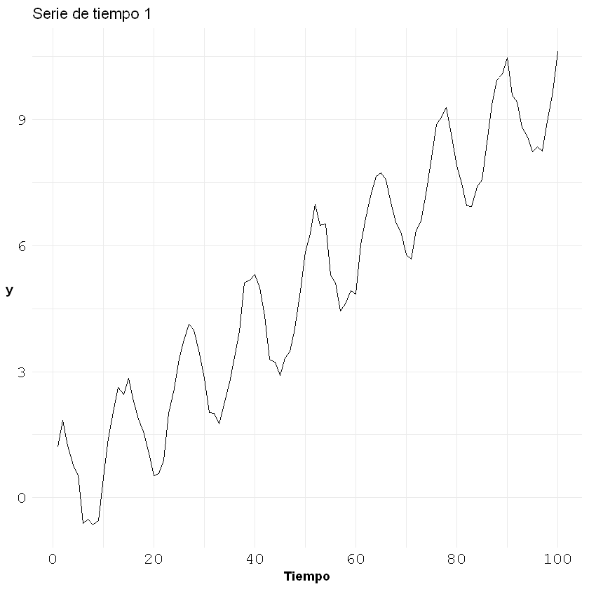
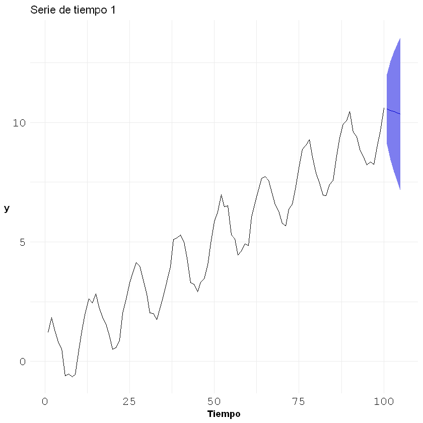
Gráfico de la serie de tiempo con el pronóstico:

Se realiza el pronóstico con la función forecast().

Para graficar solo es con autoplot(forecast). La función identifica automáticamente la serie de tiempo original y el pronóstico.

ar <- arima(estacional[,1], order = c(1, 0, 0))
forecast <- forecast(ar, h = 5, level = 99)

autoplot(forecast)+
        theme_minimal() +
        labs(title = "Serie de tiempo 1", x = "Tiempo", y = "y")+
        theme(axis.text = element_text(size = 14, family = 'mono', color = 'black'),
              axis.title.x = element_text(face = "bold", colour = "black", size = rel(1)),
              axis.title.y = element_text(face = "bold", colour = "black", size = rel(1), angle = 0,vjust = 0.5))

En forma alternativa se puede utilizar geom_forecast(h = ) y automáticamente se calculan las predicciones.

autoplot(timeserie) + geom_forecast(h = 5)+
        theme_minimal() +
        labs(title = "Serie de tiempo 1", x = "Tiempo", y = "y")+
        theme(axis.text = element_text(size = 14, family = 'mono', color = 'black'),
              axis.title.x = element_text(face = "bold", colour = "black", size = rel(1)),
              axis.title.y = element_text(face = "bold", colour = "black", size = rel(1), angle = 0,vjust = 0.5))

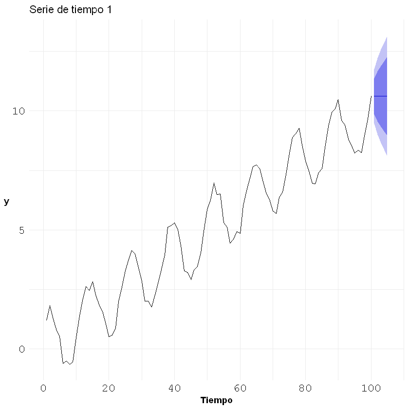
Gráfico serie de tiempo, ACF y PACF:

ggtsdisplay(timeserie)

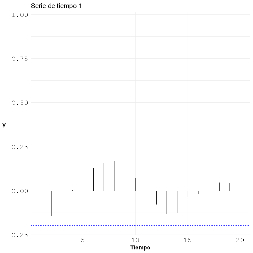
Gráfico de la ACF:

ggAcf(timeserie)+
        theme_minimal() +
        labs(title = "Serie de tiempo 1", x = "Tiempo", y = "y")+
        theme(axis.text = element_text(size = 14, family = 'mono', color = 'black'),
              axis.title.x = element_text(face = "bold", colour = "black", size = rel(1)),
              axis.title.y = element_text(face = "bold", colour = "black", size = rel(1), angle = 0,vjust = 0.5))

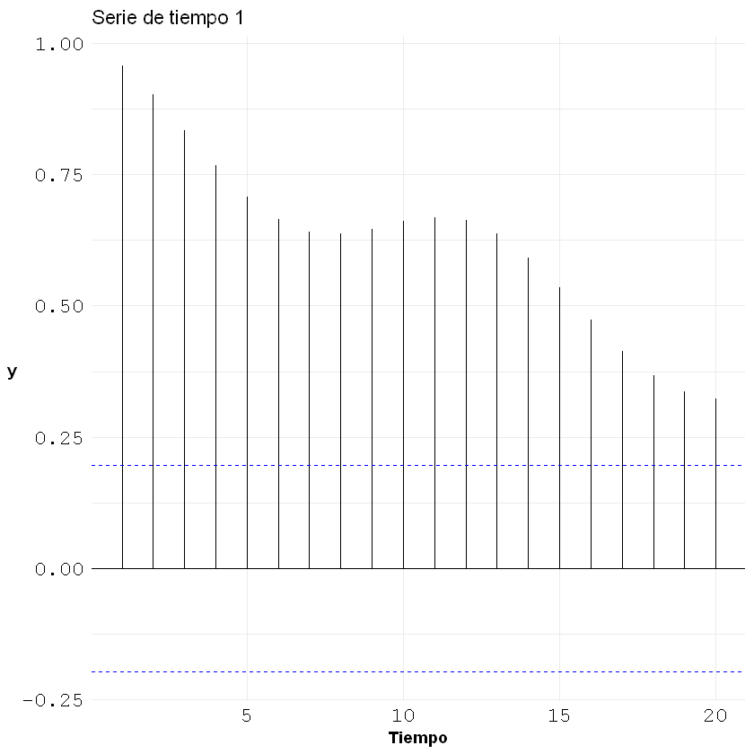
Gráfico de la PACF:

ggPacf(timeserie)+
        theme_minimal() +
        labs(title = "Serie de tiempo 1", x = "Tiempo", y = "y")+
        theme(axis.text = element_text(size = 14, family = 'mono', color = 'black'),
              axis.title.x = element_text(face = "bold", colour = "black", size = rel(1)),
              axis.title.y = element_text(face = "bold", colour = "black", size = rel(1), angle = 0,vjust = 0.5))