Regresión Logística para clasificación en R

datos = read.csv("Social_Network_Ads.csv", sep = ",", dec = ".", header = T)
print(head(datos))

   User.ID Gender Age EstimatedSalary Purchased
15624510   Male  19           19000         0
15810944   Male  35           20000         0
15668575 Female  26           43000         0
15603246 Female  27           57000         0
15804002   Male  19           76000         0
15728773   Male  27           58000         0

str(datos)

'data.frame':       400 obs. of  5 variables:
 $ User.ID        : int  15624510 15810944 15668575 15603246 15804002 15728773 15598044 15694829 15600575 15727311 ...
 $ Gender         : chr  "Male" "Male" "Female" "Female" ...
 $ Age            : int  19 35 26 27 19 27 27 32 25 35 ...
 $ EstimatedSalary: int  19000 20000 43000 57000 76000 58000 84000 150000 33000 65000 ...
 $ Purchased      : int  0 0 0 0 0 0 0 1 0 0 ...

Variables:

df <- datos[,c("Gender", "Age", "EstimatedSalary", "Purchased")]
print(head(df))

  Gender Age EstimatedSalary Purchased
 Male  19           19000         0
 Male  35           20000         0
Female  26           43000         0
Female  27           57000         0
 Male  19           76000         0
 Male  27           58000         0

print(dim(df))

[1] 400   4

Variable y:

print(table(df[,c("Purchased")]))

  0   1
257 143

print(table(df[,c("Purchased")])/nrow(df))

     0      1
0.6425 0.3575

Variable categórica:

print(unique(df$Gender))

[1] "Male"   "Female"

df$Gender <- factor(df$Gender,
                    levels = c(unique(df$Gender)),
                    labels = c(1,0))
print(head(df))

  Gender Age EstimatedSalary Purchased
    1  19           19000         0
    1  35           20000         0
    0  26           43000         0
    0  27           57000         0
    1  19           76000         0
    1  27           58000         0

Ajuste modelo múltiple:

\[p = \frac{1}{1+exp \left[- \left(\beta_0+\beta_1 \times Género +\beta_2 \times Edad + \beta_3 \times Salario \right)\right]}\]

logistic <- glm(Purchased ~ Gender + Age + EstimatedSalary, data = df, family = binomial)
logistic

Call:  glm(formula = Purchased ~ Gender + Age + EstimatedSalary, family = binomial,
    data = df)

Coefficients:
    (Intercept)          Gender0              Age  EstimatedSalary
     -1.245e+01       -3.338e-01        2.370e-01        3.644e-05

Degrees of Freedom: 399 Total (i.e. Null);  396 Residual
Null Deviance:          521.6
Residual Deviance: 275.8    AIC: 283.8

summary(logistic)

Call:
glm(formula = Purchased ~ Gender + Age + EstimatedSalary, family = binomial,
    data = df)

Deviance Residuals:
    Min       1Q   Median       3Q      Max
-2.9109  -0.5218  -0.1406   0.3662   2.4254

Coefficients:
                  Estimate Std. Error z value Pr(>|z|)
(Intercept)     -1.245e+01  1.309e+00  -9.510  < 2e-16 *
Gender0         -3.338e-01  3.052e-01  -1.094    0.274
Age              2.370e-01  2.638e-02   8.984  < 2e-16 *
EstimatedSalary  3.644e-05  5.473e-06   6.659 2.77e-11 *
---
Signif. codes:  0 '*' 0.001 '**' 0.01 '*' 0.05 '.' 0.1 ' ' 1

(Dispersion parameter for binomial family taken to be 1)

    Null deviance: 521.57  on 399  degrees of freedom
Residual deviance: 275.84  on 396  degrees of freedom
AIC: 283.84

Number of Fisher Scoring iterations: 6

Curva ROC:

Punto de corte:

Definiremos el punto de corte con la probabilidad del 70%.

Cada observación tiene una probabilidad asociada que fue ajustada por el modelo logit, logistic$fitted.values. Probabilidades mayores o iguales que 0,7 será clasificadas como $1$, es decir, que sí compraron, las demás observaciones serán clasificadas como $0$, no compraron.

y_pred <- ifelse(logistic$fitted.values >= 0.7, 1, 0)

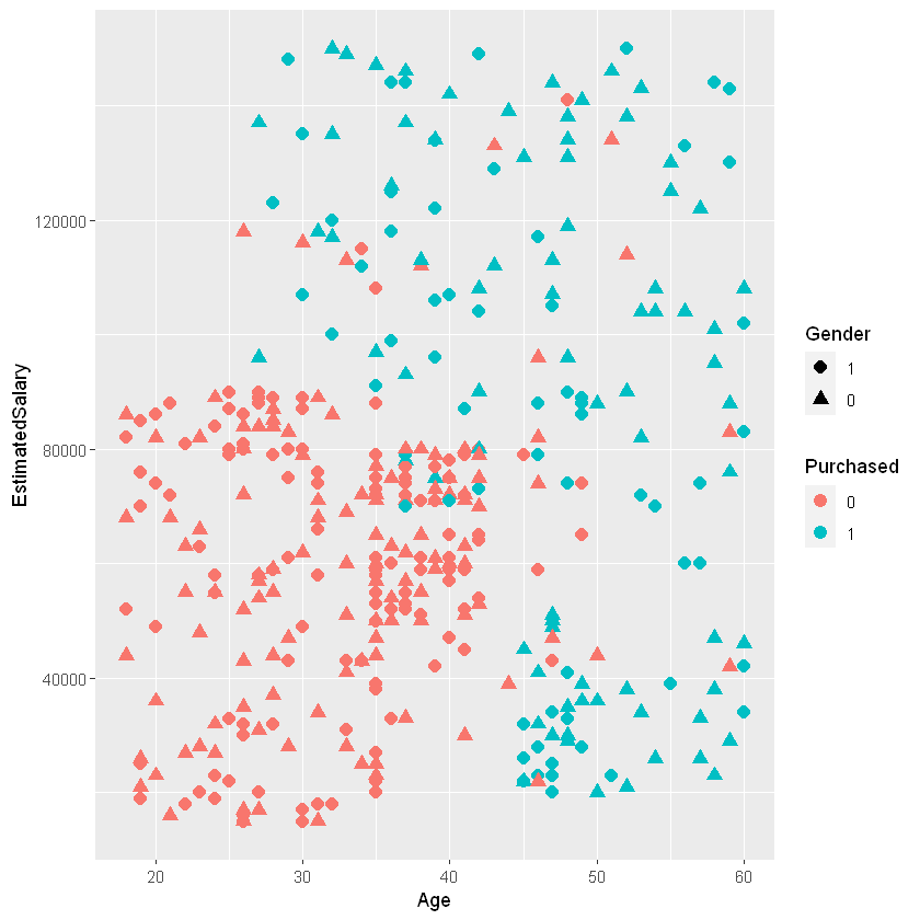
library(ggplot2)

ggplot(data = df, aes(x = Age, y = EstimatedSalary,
                      color = as.factor(Purchased), shape = Gender))+
    geom_point(size = 3)+
    labs(color = "Purchased")

Instalar el siguiente paquete: install.packages('ROCR'). Se usará la función ROCR() para graficar la curva ROC, pero primero se debe crear un objeto de predicción, se usa la función prediction() para transformar los datos en un formato estándar que se pueda graficar con la función ROCR(). Luego, se crea un objeto con el rendimiento del clasificador con la función performance(), donde se agrega el argumento measure = "tpr" para indicar True positive rate y el argumento x.measure = "fpr" para False positive rate en el eje $x$ de la curva ROC.

library(ROCR)

Warning message:
"package 'ROCR' was built under R version 4.1.3"

prediction <- prediction(y_pred, df$Purchased)
perf <- performance(prediction, measure = "tpr", x.measure = "fpr")
plot(perf)
abline(a=0, b= 1)

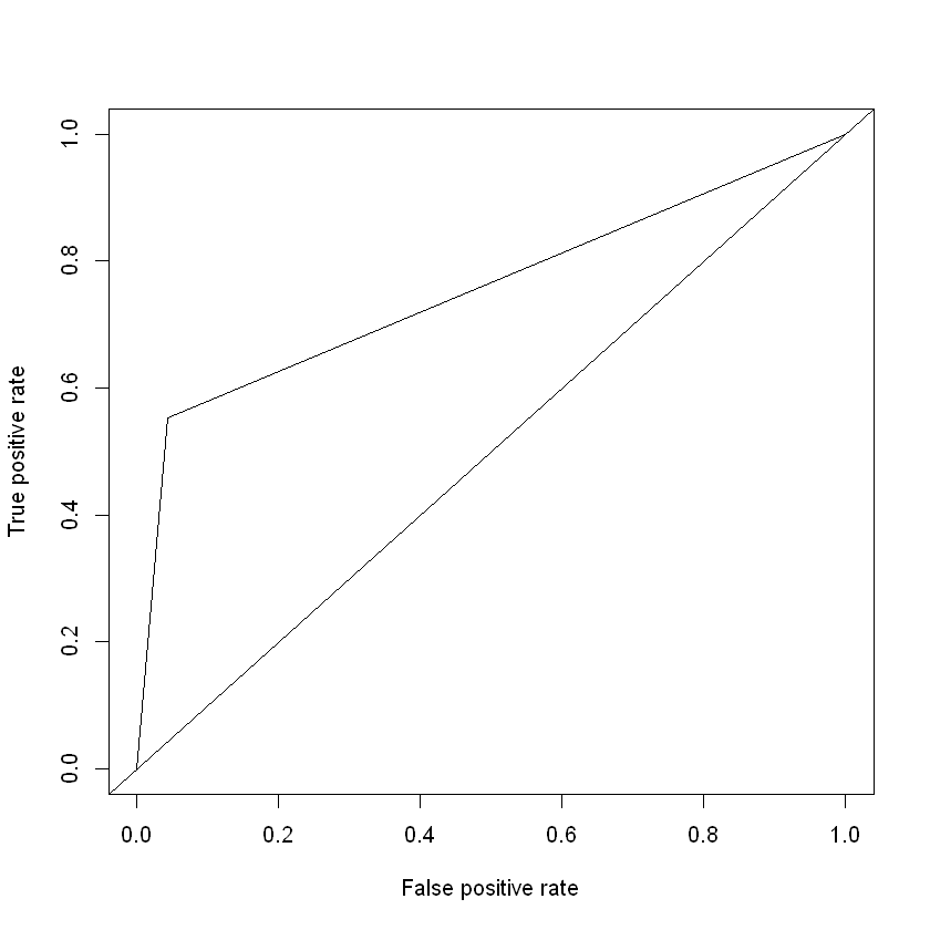
La anterior es la curva ROC para un punto de corto de 0,70.

AUC:

Podemos usar el paquete ROCR para calcular el AUC. Para hacerlo, primero debemos crear otro objeto de perf.auc, esta vez especificando measure = "auc".

perf.auc <- performance(prediction, measure = "auc")

Se usa @ porque el objeto creado tiene slots.

auc <- unlist(perf.auc@y.values)
print(auc)

[1] 0.754823

Matriz de confusión:

Antes de mostrar la matriz de confusión hagamos estos cálculos:

Cantidad de valores predichos como 1 (TP + FP):

print(sum(y_pred))

[1] 90

Cantidad de valores predichos como 0 (FN + TN):

print(length(y_pred) - sum(y_pred))

[1] 310

Cantidad de observaciones actuales que son 1:

print(sum(df$Purchased))

[1] 143

Cantidad de observaciones actuales que son 0:

print(length(df$Purchased) - sum(df$Purchased))

[1] 257

Predicciones correctas de la categoría 1 (Verdaderos Positivos - TP):

print(sum(ifelse(df$Purchased == 1 & y_pred == 1, 1, 0)))

[1] 79

Predicciones correctas para la categoría 0 (Verdaderos Negativos - TN):

print(sum(ifelse(df$Purchased == 0 & y_pred == 0, 1, 0)))

[1] 246

Predicciones correctas en total:

print(sum(ifelse(df$Purchased == y_pred, 1,0)))

[1] 325

Cantidad de predicciones incorrectas para la categoría 1 (Falso negativo - FN - Error tipo 2):

print(sum(ifelse(df$Purchased == 1 & y_pred == 0, 1, 0)))

[1] 64

Cantidad de predicciones incorrectas para la categoría 0 (Falso positivo - FP - Error tipo 1):

print(sum(ifelse(df$Purchased == 0 & y_pred == 1, 1, 0)))

[1] 11

La siguiente matriz de confusión tiene la forma:

	Predicho como 0	Predicho como 1
Actual 0	TN	FP
Actual 1	FN	TP

cm <- table(df$Purchased, y_pred)
print(cm)

 y_pred
 1
246  11
64  79

Métricas:

TP <- cm[4]
print(TP)

[1] 79

TN <- cm[1]
print(TN)

[1] 246

FN <- cm[2]
print(FN)

[1] 64

FP <- cm[3]
print(FP)

[1] 11

print(sum(cm))

[1] 400

Accuracy:

\[accuracy = \frac{TP+TN}{TP+TN+FP+FN}\]

accuracy <- (TP+TN)/sum(cm)
print(accuracy)

[1] 0.8125

Error Rate:

\[ErrorRate = \frac{FP+FN}{TP+TN+FP+FN} = 1 - accuracy\]

error <- (FP+FN)/sum(cm)
print(error)

[1] 0.1875

Sensitivity:

\[sensitivity = \frac{TP}{TP+FN}\]

sensitivity <- TP/(TP+FN)
print(sensitivity)

[1] 0.5524476

Specificity:

\[specificity = \frac{TN}{TN+FP}\]

specificity <- TN/(TN+FP)
print(specificity)

[1] 0.9571984

Precision:

\[precision = \frac{TP}{TP+FP}\]

precision <- TP/(TP+FP)
print(precision)

[1] 0.8777778

Recall:

\[recall = \frac{TP}{TP+FN}\]

recall <- TP/(TP+FN)
print(recall)

[1] 0.5524476

F-measure:

\[F-measure = \frac{2 \times precision \times recall}{recall + precision} = \frac{2 \times TP}{2 \times TP + FP + FN}\]

F1 <- (2*precision*recall)/(recall+precision)
print(F1)

[1] 0.6781116

F1 <- (2*TP)/(2*TP+FP+FN)
print(F1)

[1] 0.6781116

¿Cómo cambian los resultados si el punto de corte es con una probabilidad de 0,50?