Ejemplo de Análisis de correspondencia: Simple y Múltiple
Análisis simple
datos<- read.csv("registro_artesanos.csv", sep=";",header=T)
(head(datos))
| edad | sexo | cabeza_de_hogar | caracterizacion_ciudadano | tipo_de_emprendimiento | idea_de_negocio | estrato | barrio_vereda_ciudadano | comuna_ciudadano | zona_ciudadano | fecha_de_beneficio_dia | fecha_de_beneficio_mes | fecha_de_beneficio_aÃ.o | |
|---|---|---|---|---|---|---|---|---|---|---|---|---|---|
| <int> | <chr> | <chr> | <chr> | <chr> | <chr> | <int> | <chr> | <chr> | <chr> | <int> | <int> | <dbl> | |
| 1 | 63 | masculino | si | emprendedor | artesanal | emprendedor | 2 | robledo | 7 | nor-occidental | 15 | 9 | 2017 |
| 2 | 56 | masculino | no | emprendedor | artesanal | emprendedor | 3 | bombona | 10 | centro-oriental | 15 | 9 | 2017 |
| 3 | 74 | masculino | si | emprendedor | artesanal | emprendedor | 3 | guayabal | 15 | sur-oriental | 15 | 9 | 2017 |
| 4 | 54 | femenino | si | emprendedor | artesanal | emprendedor | 4 | america - santa monica #2 | 12 | centro-oriental | 15 | 9 | 2017 |
| 5 | 50 | femenino | si | emprendedor | artesanal | emprendedor | 4 | america - santa monica #2 | 12 | centro-oriental | 15 | 9 | 2017 |
| 6 | 52 | femenino | si | emprendedor | artesanal | emprendedor | 3 | san javier | 13 | centro-oriental | 15 | 9 | 2017 |
#eliminando NAs
datos <- na.omit(datos)
str(datos)
'data.frame':       174 obs. of  13 variables:
 $ edad                     : int  63 56 74 54 50 52 27 61 43 39 ...
 $ sexo                     : chr  "masculino" "masculino" "masculino" "femenino" ...
 $ cabeza_de_hogar          : chr  "si" "no" "si" "si" ...
 $ caracterizacion_ciudadano: chr  "emprendedor" "emprendedor" "emprendedor" "emprendedor" ...
 $ tipo_de_emprendimiento   : chr  "artesanal" "artesanal" "artesanal" "artesanal" ...
 $ idea_de_negocio          : chr  "emprendedor" "emprendedor" "emprendedor" "emprendedor" ...
 $ estrato                  : int  2 3 3 4 4 3 3 3 2 2 ...
 $ barrio_vereda_ciudadano  : chr  "robledo" "bombona" "guayabal" "america - santa monica #2" ...
 $ comuna_ciudadano         : chr  "7" "10" "15" "12" ...
 $ zona_ciudadano           : chr  "nor-occidental" "centro-oriental" "sur-oriental" "centro-oriental" ...
 $ fecha_de_beneficio_dia   : int  15 15 15 15 15 15 15 15 15 15 ...
 $ fecha_de_beneficio_mes   : int  9 9 9 9 9 9 9 9 9 9 ...
 $ fecha_de_beneficio_aÃ.o  : num  2017 2017 2017 2017 2017 ...
 - attr(, "na.action")= 'omit' Named int [1:25] 112 122 125 127 131 136 137 138 139 140 ...
  ..- attr(, "names")= chr [1:25] "112" "122" "125" "127" ...
Extraemos las variables de interés
df<- datos[,c("tipo_de_emprendimiento","zona_ciudadano")]
print(head(df))
  tipo_de_emprendimiento  zona_ciudadano
1              artesanal  nor-occidental
2              artesanal centro-oriental
3              artesanal    sur-oriental
4              artesanal centro-oriental
5              artesanal centro-oriental
6              artesanal centro-oriental
Creamos tabla de contingencia
contingencia<-table(df)
print(contingencia)
                      zona_ciudadano
tipo_de_emprendimiento    centro-occidental centro-oriental nor-occidental
                        0                 4               0              0
            artesanal   0                 0              51             18
            artesanias  2                14               4             14
            basica      0                 1               0              1
            no formal   0                 1               0              0
            no_formal   0                 0               0              0
                      zona_ciudadano
tipo_de_emprendimiento nor-oriental occidente oriente otro sur-occidental
                                  2         0       0    2              1
            artesanal            16         3       5    0              2
            artesanias            8         0       0    5             13
            basica                0         0       0    1              0
            no formal             0         0       0    0              0
            no_formal             1         0       0    0              0
                      zona_ciudadano
tipo_de_emprendimiento sur-oriental
                                  0
            artesanal             5
            artesanias            0
            basica                0
            no formal             0
            no_formal             0
Se realiza gráfico de contingencias
library(gplots)
Warning message:
"package 'gplots' was built under R version 4.1.3"

Attaching package: 'gplots'


The following object is masked from 'package:stats':

    lowess
balloonplot(t(contingencia), main ="Caracterización",
            xlab = "", ylab= "",
            label = T,
            show.margins = T)

Test de independencia
library(pander)
Warning message:
"package 'pander' was built under R version 4.1.3"
print(pander(chisq.test(contingencia)))
Warning message in chisq.test(contingencia):
"Chi-squared approximation may be incorrect"
| Test statistic | df |     P value     |
|:--------------:|:--:|:---------------:|
|      120       | 45 | 9.49e-09  * * * |

Table: Pearson's Chi-squared test: contingencia

NULL
Extracción por AC
library(FactoMineR)
library(factoextra)
Warning message:
"package 'FactoMineR' was built under R version 4.1.3"
Warning message:
"package 'factoextra' was built under R version 4.1.3"
Loading required package: ggplot2

Welcome! Want to learn more? See two factoextra-related books at https://goo.gl/ve3WBa
CA_simple<- CA(contingencia)
print(CA_simple)
Results of the Correspondence Analysis (CA)
The row variable has  6  categories; the column variable has 10 categories
The chi square of independence between the two variables is equal to 120.0362 (p-value =  9.489902e-09 ).
*The results are available in the following objects:

   name              description
1  "$eig"            "eigenvalues"
2  "$col"            "results for the columns"
3  "$col$coord"      "coord. for the columns"
4  "$col$cos2"       "cos2 for the columns"
5  "$col$contrib"    "contributions of the columns"
6  "$row"            "results for the rows"
7  "$row$coord"      "coord. for the rows"
8  "$row$cos2"       "cos2 for the rows"
9  "$row$contrib"    "contributions of the rows"
10 "$call"           "summary called parameters"
11 "$call$marge.col" "weights of the columns"
12 "$call$marge.row" "weights of the rows"
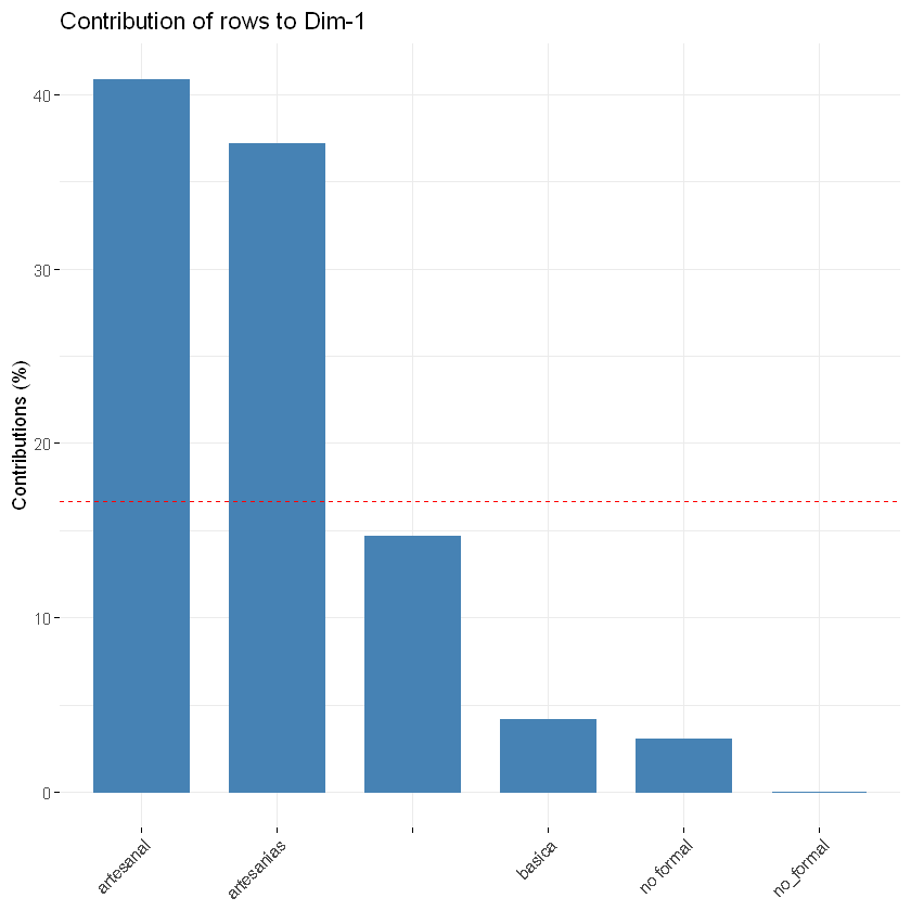
Obtenemos y analizamos contribuciones columnas
fviz_contrib(CA_simple, choice = "col", axes = 1)

print(CA_simple$col$contrib)
                        Dim 1      Dim 2        Dim 3       Dim 4      Dim 5
V1                 2.27549859 12.9234349  0.003035806  0.05651337  0.1500657
centro-occidental 33.33699063 15.9974851  0.880836721 36.26967998  2.0207547
centro-oriental   28.94593235  1.7096477  4.427712262  2.06995300  7.3975893
nor-occidental     0.02716778 12.7449870 10.812273634  5.60234253 46.8617649
nor-oriental       0.14822371  0.9281056 78.121151270  2.30533427  2.9799437
occidente          2.24995127  0.4551492  0.275299399  0.11528355  0.5216493
oriente            3.74991878  0.7585820  0.458832331  0.19213924  0.8694156
otro              13.50375554 17.7702438  4.156448465 53.03715929  5.7259774
sur-occidental    12.01264257 35.9537829  0.405577782  0.15945552 32.6034237
sur-oriental       3.74991878  0.7585820  0.458832331  0.19213924  0.8694156
fviz_contrib(CA_simple, choice = "row", axes = 1)
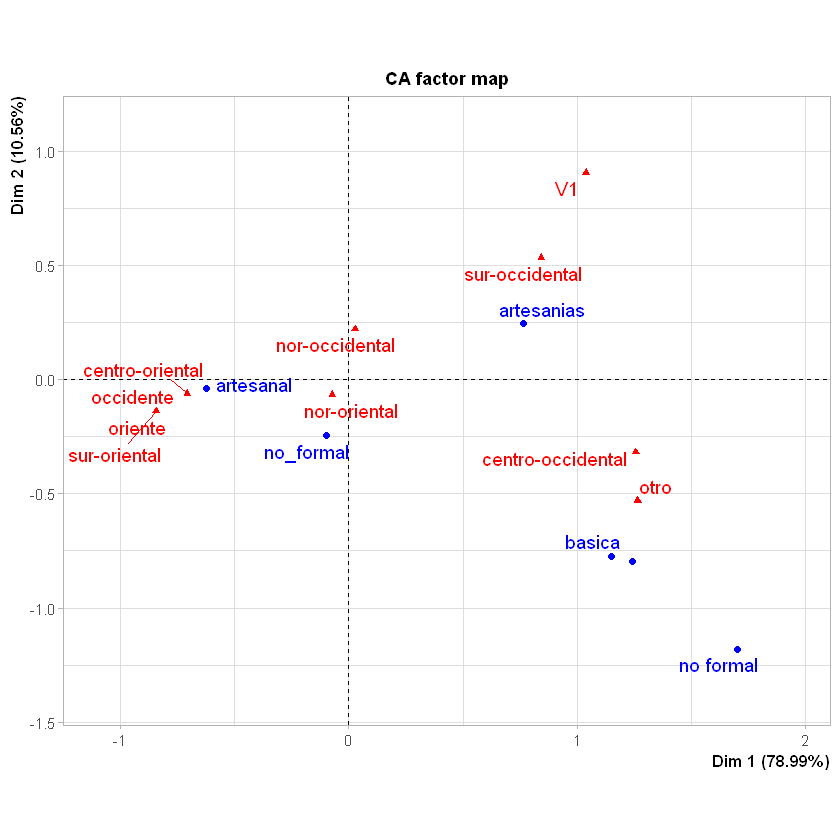
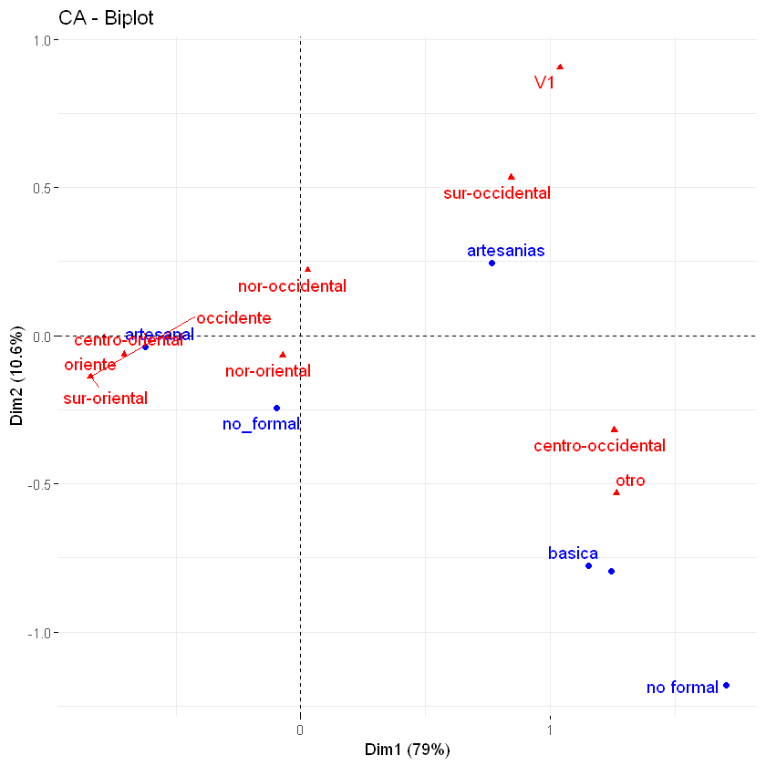
Representación en el biplot
fviz_ca_biplot(CA_simple, repel = TRUE)
Múltiple
df_m<- datos[,c("tipo_de_emprendimiento","zona_ciudadano","cabeza_de_hogar","sexo")]
print(head(df_m))
  tipo_de_emprendimiento  zona_ciudadano cabeza_de_hogar      sexo
1              artesanal  nor-occidental              si masculino
2              artesanal centro-oriental              no masculino
3              artesanal    sur-oriental              si masculino
4              artesanal centro-oriental              si  femenino
5              artesanal centro-oriental              si  femenino
6              artesanal centro-oriental              si  femenino
Ajuste ACM
CA_multiple <- MCA(df_m,method = 'Burt')
summary(CA_multiple)
Warning message:
"ggrepel: 3 unlabeled data points (too many overlaps). Consider increasing max.overlaps"
Call:
MCA(X = df_m, method = "Burt")
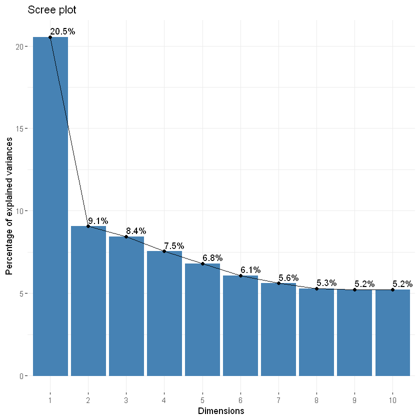
Eigenvalues
Dim.1 Dim.2 Dim.3 Dim.4 Dim.5 Dim.6 Dim.7
Variance 0.245 0.108 0.101 0.090 0.081 0.073 0.067
% of var. 20.543 9.055 8.444 7.547 6.796 6.070 5.599
Cumulative % of var. 20.543 29.598 38.042 45.589 52.385 58.455 64.054
Dim.8 Dim.9 Dim.10 Dim.11 Dim.12 Dim.13 Dim.14
Variance 0.063 0.063 0.062 0.054 0.047 0.044 0.042
% of var. 5.280 5.231 5.231 4.545 3.917 3.689 3.490
Cumulative % of var. 69.334 74.566 79.797 84.341 88.259 91.948 95.437
Dim.15 Dim.16 Dim.17
Variance 0.029 0.021 0.004
% of var. 2.458 1.767 0.338
Cumulative % of var. 97.895 99.662 100.000
Individuals (the 10 first)
Dim.1 ctr cos2 Dim.2 ctr cos2
1 | -0.671 0.522 0.221 | 0.075 0.010 0.003
2 | -0.700 0.568 0.300 | -0.428 0.320 0.112
3 | -0.942 1.030 0.094 | -0.462 0.373 0.023
4 | -0.584 0.396 0.331 | -0.091 0.015 0.008
5 | -0.584 0.396 0.331 | -0.091 0.015 0.008
6 | -0.584 0.396 0.331 | -0.091 0.015 0.008
7 | 0.030 0.001 0.001 | -0.287 0.144 0.049
8 | -0.457 0.243 0.085 | 0.310 0.167 0.039
9 | 0.030 0.001 0.001 | -0.287 0.144 0.049
10 | -0.099 0.011 0.001 | -1.054 1.940 0.123
Dim.3 ctr cos2
1 | -0.224 0.091 0.025 |
2 | -0.107 0.021 0.007 |
3 | -0.029 0.001 0.000 |
4 | 0.191 0.066 0.035 |
5 | 0.191 0.066 0.035 |
6 | 0.191 0.066 0.035 |
7 | -0.322 0.188 0.062 |
8 | 0.166 0.050 0.011 |
9 | -0.322 0.188 0.062 |
10 | -0.200 0.072 0.004 |
Categories (the 10 first)
Dim.1 ctr cos2 v.test Dim.2 ctr
tipo_de_emprendimiento_ | 0.894 4.211 0.154 2.746 | 0.009 0.001
tipo_de_emprendimiento_artesanal | -0.519 15.776 0.888 -7.937 | -0.124 2.033
tipo_de_emprendimiento_artesanias | 0.657 15.180 0.634 6.273 | 0.223 3.960
tipo_de_emprendimiento_basica | 0.963 1.629 0.061 1.678 | -0.675 1.813
tipo_de_emprendimiento_no formal | 1.693 1.677 0.063 1.693 | -2.144 6.103
tipo_de_emprendimiento_no_formal | -0.161 0.015 0.001 -0.161 | 3.085 12.640
zona_ciudadano_ | 0.535 0.335 0.013 0.759 | 0.570 0.862
zona_ciudadano_centro-occidental | 1.099 14.152 0.486 5.211 | -0.395 4.152
zona_ciudadano_centro-oriental | -0.621 12.433 0.548 -5.557 | -0.175 2.235
zona_ciudadano_nor-occidental | 0.016 0.005 0.000 0.099 | 0.027 0.032
cos2 v.test Dim.3 ctr cos2 v.test
tipo_de_emprendimiento_ 0.000 0.028 | 1.430 26.209 0.393 4.393 |
tipo_de_emprendimiento_artesanal 0.050 -1.892 | 0.031 0.136 0.003 0.473 |
tipo_de_emprendimiento_artesanias 0.073 2.127 | -0.376 12.081 0.207 -3.588 |
tipo_de_emprendimiento_basica 0.030 -1.175 | 1.277 6.966 0.108 2.225 |
tipo_de_emprendimiento_no formal 0.101 -2.144 | 0.705 0.708 0.011 0.705 |
tipo_de_emprendimiento_no_formal 0.212 3.085 | 2.060 6.041 0.094 2.060 |
zona_ciudadano_ 0.015 0.808 | -1.546 6.807 0.108 -2.193 |
zona_ciudadano_centro-occidental 0.063 -1.874 | 0.296 2.488 0.035 1.401 |
zona_ciudadano_centro-oriental 0.043 -1.564 | 0.065 0.327 0.006 0.578 |
zona_ciudadano_nor-occidental 0.001 0.171 | -0.336 5.294 0.103 -2.136 |
Categorical variables (eta2)
Dim.1 Dim.2 Dim.3
tipo_de_emprendimiento | 0.763 0.349 0.662 |
zona_ciudadano | 0.769 0.628 0.548 |
cabeza_de_hogar | 0.173 0.338 0.050 |
sexo | 0.277 0.000 0.011 |
Extrayendo los valores propios
eig.val = get_eigenvalue(CA_multiple)
eig.val
| eigenvalue | variance.percent | cumulative.variance.percent | |
|---|---|---|---|
| Dim.1 | 0.245442118 | 20.543086 | 20.54309 |
| Dim.2 | 0.108187325 | 9.055094 | 29.59818 |
| Dim.3 | 0.100886345 | 8.444015 | 38.04219 |
| Dim.4 | 0.090164207 | 7.546590 | 45.58878 |
| Dim.5 | 0.081194727 | 6.795860 | 52.38464 |
| Dim.6 | 0.072525536 | 6.070263 | 58.45491 |
| Dim.7 | 0.066895904 | 5.599073 | 64.05398 |
| Dim.8 | 0.063089070 | 5.280447 | 69.33443 |
| Dim.9 | 0.062500000 | 5.231143 | 74.56557 |
| Dim.10 | 0.062500000 | 5.231143 | 79.79671 |
| Dim.11 | 0.054298259 | 4.544672 | 84.34139 |
| Dim.12 | 0.046802939 | 3.917326 | 88.25871 |
| Dim.13 | 0.044074548 | 3.688964 | 91.94768 |
| Dim.14 | 0.041695178 | 3.489815 | 95.43749 |
| Dim.15 | 0.029366877 | 2.457957 | 97.89545 |
| Dim.16 | 0.021105663 | 1.766508 | 99.66196 |
| Dim.17 | 0.004038829 | 0.338043 | 100.00000 |
Gráfico de sedimentación para identificar dimensiones óptimas
fviz_screeplot(CA_multiple, addlabels = TRUE)
Ubicación en el biplot como representación de las dimensiones
fviz_mca_biplot(CA_multiple, repel = TRUE)
Warning message:
"ggrepel: 121 unlabeled data points (too many overlaps). Consider increasing max.overlaps"
