LSTM
import pandas as pd
import numpy as np
import matplotlib.pyplot as plt
from keras.models import Sequential
from keras.layers import Dense, SimpleRNN, LSTM, Dropout
from sklearn.preprocessing import MinMaxScaler
from sklearn.metrics import mean_squared_error, r2_score
from sklearn import linear_model
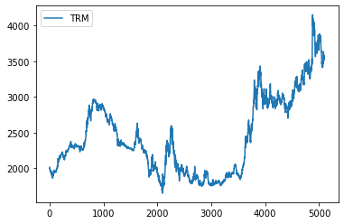
data = pd.read_csv("TRM.csv", sep = ";", decimal=",")
dataNorm = data.drop(['Fecha'], 1, inplace=True)
data.plot()
plt.show()
Conjunto de Train y Test:
200 precios como test.
train = data.values[:len(data) - 200]
test = data.values[len(data) - 200:]
Creación datos de entrada a la red:
Los datos de entrada a la red tienen que tener la forma de 3D tensor:
\[[samples, timesteps, features]\]
La siguiente función crea los times steps.
def batch(data, timeSteps):
 X, Y =[], []
 for i in range(len(data)-timeSteps):
  j=i+timeSteps
  X.append(data[i:j,0])
  Y.append(data[j,0])
 return np.array(X), np.array(Y)
Time steps de 5 y features de 1, es decir, se utilizarán 5 precios históricos para predecir 1 precio.
X_train, y_train = batch(train, 5)
X_test, y_test = batch(test, 5)
Transformación de los datos en 3D tensor:
X_train = np.reshape(X_train, (X_train.shape[0], X_train.shape[1], 1))
X_test = np.reshape(X_test, (X_test.shape[0], X_test.shape[1], 1))
RNN:
model = Sequential()
model.add(SimpleRNN(units = 10, activation = "relu", input_shape=(5,1)))
model.add(Dropout(0.2))
model.add(Dense(1))
model.compile(optimizer = 'adam', loss = 'mean_squared_error')
history = model.fit(X_train, y_train, validation_data=(X_test, y_test), batch_size = 20, epochs = 10, verbose=0)
Comparación Loss training vs. Loss testing:
epochs = range(1, 10 + 1)
loss = history.history["loss"]
valLoss = history.history["val_loss"]

plt.plot(epochs, loss, "b", label = "Training Loss", color = "blue")
plt.plot(epochs, valLoss, "b", label = "Testing Loss", color = "red")
plt.title("Model Loss")
plt.legend()
plt.show()

y_test_pred_RNN = model.predict(X_test)
y_test_pred_RNN = sc.inverse_transform(y_test_pred_RNN.reshape(-1,1))
y_true = sc.inverse_transform(y_test.reshape(-1,1))
MSE
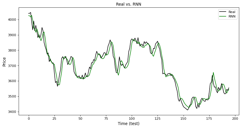
mean_squared_error(y_true, y_test_pred_RNN)
1117.1567997692296
plt.figure(figsize=(12, 6), dpi=80, facecolor = 'w', edgecolor = 'k')

plt.plot(y_true, color='black', label='Real')
plt.plot(y_test_pred_RNN, color = 'green', label = 'RNN')

plt.title('Real vs. RNN', fontsize = 12)
plt.xlabel('Time (test)', fontsize=12)
plt.ylabel('Price', fontsize = 12)
plt.legend(loc = 'best')
plt.show()
Ajuste de regresión
regressor = linear_model.LinearRegression()
regressor.fit(y_true, y_test_pred_RNN)
LinearRegression()
print('R2: %.2f' % r2_score(y_true, y_test_pred_RNN))
R2: 0.95
LSTM:

1
Una capa de 10 celdas LSTM.
Función de activación: ReLu.
Batch size: 20.
Epochs: 10.
Dropout: 20% para evitar overfitting.
model = Sequential()
model.add(LSTM(units = 10, activation = "relu", input_shape=(5,1)))
model.add(Dropout(0.2))
model.add(Dense(1))
model.compile(optimizer = 'adam', loss = 'mean_squared_error')
history = model.fit(X_train, y_train, validation_data=(X_test, y_test), batch_size = 20, epochs = 10, verbose=0)
Comparación Loss training vs. Loss testing:
epochs = range(1, 10 + 1)
loss = history.history["loss"]
valLoss = history.history["val_loss"]

plt.plot(epochs, loss, "b", label = "Training Loss", color = "blue")
plt.plot(epochs, valLoss, "b", label = "Testing Loss", color = "red")
plt.title("Model Loss")
plt.legend()
plt.show()

y_test_pred_LSTM = model.predict(X_test)
y_test_pred_LSTM = sc.inverse_transform(y_test_pred_LSTM.reshape(-1,1))
MSE
mean_squared_error(y_true, y_test_pred_LSTM)
2618.8473693593573
plt.figure(figsize=(12, 6), dpi=80, facecolor = 'w', edgecolor = 'k')

plt.plot(y_true, color='black', label='Real')
plt.plot(y_test_pred_LSTM, color = 'green', label = 'LSTM')

plt.title('Real vs. LSTM', fontsize = 12)
plt.xlabel('Time (test)', fontsize=12)
plt.ylabel('Price', fontsize = 12)
plt.legend(loc = 'best')
plt.show()

Ajuste de regresión
regressor = linear_model.LinearRegression()
regressor.fit(y_true, y_test_pred_LSTM)
LinearRegression()
print('R2: %.2f' % r2_score(y_true, y_test_pred_LSTM))
R2: 0.88